If you’re planning a cooling retrofit (RDHx, direct-to-chip liquid, or a hybrid zone) the hard part isn’t the physics—it’s getting finance, facilities, and operations to agree on a cost model they’ll actually sign.
This step-by-step guide gives you a defensible way to estimate 24–36 month total cost of ownership (TCO) and ROI/payback for retrofit options using four input families:
Energy (IT load, PUE change, $/kWh, and a simple demand-charge sensitivity)
Maintenance (what goes away, what gets added, and how to model labor + contracts)
Capex bands (RDHx vs. DLC, plus install/commissioning)
Water costs (WUE and blended water + sewer rates)
Key Takeaway: A retrofit ROI model is only as credible as its baseline. Use measured 12-month inputs where possible, then run sensitivity bands—don’t sell a single-point “payback number.”
What you’ll have when you’re done
By the end of Step 9, you’ll be able to produce:
24- and 36-month cash flows for a “do nothing” baseline vs. retrofit options
Simple payback and ROI (and optional NPV)
A sensitivity view that shows which variable actually drives the decision
Prerequisites and scope boundaries
Before you start, decide what is in-scope for your model:
Scope A (recommended for 24–36 months): cooling energy + cooling maintenance + water + retrofit capex
Scope B (optional if you can quantify it): avoided downtime risk, extended hardware life, and capacity/space value
Keep Scope B as a separate line item unless you can defend the assumptions under scrutiny.
Step 1: Lock the baseline (inputs) you’re willing to defend
Data center cooling retrofit ROI: the inputs that drive results
Before you debate vendors or architectures, align on what your model will treat as drivers vs. assumptions. This is the fastest way to keep the conversation about validation, not opinions.
This is also where a PUE improvement ROI model either becomes credible (measured baselines + transparent ranges) or collapses (guessed baselines + one-point outcomes).
Inputs
Average and peak IT load (kW) for the zone you’re retrofitting
Baseline PUE for that zone or the closest measurable proxy
Electricity tariff: $/kWh and any known demand charge ($/kW-month)
Current cooling O&M costs (labor hours, filters, CRAC/CRAH service contracts)
Baseline water (annual gallons) or baseline data center WUE if you track it
Action
Use 12 months of metered data if you have it (seasonality matters).
If you only have facility-level PUE, document that you’re modeling “facility blended” savings and applying a conservative factor to the retrofit zone.
Outputs
A baseline input sheet with a source note for each variable (meter, CMMS, utility bill, assumption)
Done when…
Every baseline variable is traceable to a document or a stated assumption.
Step 2: Define the retrofit options and what changes operationally
Inputs
Option set (example):
Option 1: RDHx (rear-door heat exchanger) for a defined rack row/zone (use this to model rear-door heat exchanger (RDHx) payback)
Option 2: DLC (direct-to-chip / cold plate) for a GPU/HPC pod (use this to model direct liquid cooling (DLC) TCO)
Option 3: Hybrid (RDHx + targeted DLC)
Action For each option, write a one-paragraph “what changes” statement:
What gets added (water loop interfaces, CDUs, leak detection, monitoring, commissioning)
What gets reduced (fan power, airflow rework, filters, hot-spot firefighting)
What stays the same (upstream plant constraints, redundancy requirements, controls ownership)
Outputs
Option definitions that facilities + operations agree are accurate
Done when…
You can hand this to an ops lead and they say, “Yes—that’s what we’ll have to run.”
Step 3: Set capex bands (RDHx vs. DLC) and make them comparable
Inputs
Capex bands by option (you can start with bands, then replace with quotes later)
Installation and commissioning scope (night work, phasing, containment changes, controls integration)
Action Structure capex in a way that stops arguments:
Equipment (RDHx doors / CDUs / manifolds / sensors)
Mechanical + piping (valves, hoses, quick connects, insulation)
Electrical + controls (power, BMS integration, alarms)
Commissioning (functional tests, acceptance criteria, training)
If you want a quick, defendable starting point for retrofit economics, Coolnet’s containment ROI article includes a worked payback example and cost ranges you can use as a reference framing (not a quote): Coolnet’s quick ROI math and commissioning checklist.
Outputs
Capex totals per option, plus a clear “included vs. excluded” list
Done when…
Procurement can see what’s missing, and engineering can see what’s included.
Step 4: Model energy costs using a PUE-based method (and keep it conservative)
Inputs
IT load (kW)
Baseline PUE and post-retrofit PUE (or a conservative delta)
Electricity energy price ($/kWh)
Action Use a simple, auditable approach:
Annual facility energy (kWh) ≈ IT kW × PUE × 8,760
Annual energy cost ($) ≈ Annual facility kWh × $/kWh
Then calculate savings from the PUE delta:
Annual energy savings ($) ≈ IT kW × (PUE_before − PUE_after) × 8,760 × $/kWh
Pro Tip: If you don’t have a credible post-retrofit PUE estimate yet, model three PUE cases (conservative/base/aggressive) and let the sensitivity chart do the arguing.
Outputs
Annual energy cost baseline vs. each option
Annual energy savings per option (banded)
Done when…
Someone can change only PUE and $/kWh and see the model behave correctly.
Step 5: Add a demand-charge sensitivity without overcomplicating the model
Inputs
Demand charge rate ($/kW-month) if known
Your best estimate of peak reduction (kW) from the retrofit (or a percent band)
Action If your tariff includes demand charges, treat them as a sensitivity band unless you can model peaks precisely.
A simple approach:
Annual demand savings ($) ≈ Peak kW reduction × demand rate × 12
If you don’t know peak reduction, run a sensitivity band (e.g., 0%, 2%, 5% of the affected load). For a plain-language explanation of how demand charges work, see a simple explanation of utility demand charges.
Outputs
Incremental annual savings band from demand charges
Done when…
Finance agrees demand is treated as a sensitivity (not a hidden assumption).
Step 6: Model maintenance (what you remove, what you add)
Inputs
Current annual cooling maintenance costs ($) and/or labor hours
New maintenance elements per option (pumps/CDU maintenance, leak detection checks, filter reductions)
Action Split maintenance into two buckets:
Avoided air-side O&M: filters, fan arrays, recurring hot-spot investigations, rebalancing
Added liquid-side O&M: pump checks, fluid sampling (if applicable), sensor calibration, leak response drills
Use conservative defaults if you lack historical data:
Start with a maintenance reduction band (e.g., 10–30% for a modest retrofit; higher only if you can defend it)
Add a fixed line item for liquid-side checks rather than assuming “maintenance goes to zero”
Outputs
Annual maintenance cost baseline vs. each option
A short narrative explaining the maintenance delta (helps during approval)
Done when…
Operations signs off that the model reflects real work, not marketing.
Step 7: Convert water and WUE into dollars (and disclose scope)
Inputs
Baseline annual water usage (gallons) or baseline WUE
Blended water + sewer rate ($/1,000 gallons) where applicable
Post-retrofit water assumption (may be unchanged for closed-loop options; may change if you alter tower operation)
Action Use standardized definitions and document scope.
The U.S. DOE FEMP outlines common data center water-efficiency approaches and provides baseline formulas for PUE and WUE in its guidance on data center cooling water efficiency opportunities.
Practical modeling tips:
Treat water as a sensitivity driver unless you have metering at the right boundary.
Don’t mix “cooling tower makeup water” with “site water” without stating what you’re measuring.
Outputs
Annual water cost baseline vs. each option (or “no change” with rationale)
Done when…
Your water savings claim matches what you can actually meter and report.
Step 8: Build 24- and 36-month cash flows (not just annual savings)
Inputs
Capex timing (month 0 or phased)
Annual savings by category (energy, demand, maintenance, water)
Action Convert annual savings into monthly cash flows:
Monthly savings ≈ annual savings / 12
Cash flow timeline:
Month 0: capex outflow (or phased capex)
Months 1–36: savings inflows
Outputs
24-month and 36-month net cash position by option
Done when…
Anyone can see exactly when (and why) the line crosses zero.
Step 9: Calculate payback, ROI, and (optional) NPV
Inputs
Total capex per option
Total net savings per year (or over 24/36 months)
Action Use simple formulas first:
Simple payback (years) = Capex / Annual net savings
ROI over 24 months = (24-month net savings − capex) / capex
ROI over 36 months = (36-month net savings − capex) / capex
If finance expects it, add NPV with a discount rate (and keep the rate explicit).
Outputs
Payback (months)
ROI at 24 and 36 months
Optional NPV
Done when…
Your ROI summary ties directly back to the cash flow sheet (no “magic” cells).
Step 10: Run sensitivity cases (base/best/worst + a mini tornado)
Inputs Pick 4–6 variables that actually matter:
$/kWh
PUE_before and PUE_after (or ΔPUE)
Capex band (RDHx and DLC)
Demand-charge impact (0–5% peak reduction band)
Water rate and WUE assumption
Maintenance delta
Action Create three cases:
Conservative: low savings, high capex, low utility rates
Base: best available assumptions
Upside: higher utility rates and higher verified savings (not “marketing max”)
Then rank variables by ROI impact (a simple tornado chart works well).
Outputs
Case table (conservative/base/upside)
A ranked list of what actually drives payback
Done when…
The decision conversation shifts from opinion to “which variable do we validate next?”
Common failure modes (and how to avoid them)
Baseline isn’t real. If you’re using assumed PUE/WUE, label it and run conservative bands.
Capex is missing commissioning and controls. Retrofits fail in the handoff, not the CAD.
Maintenance savings are overstated. Make sure “what gets added” is in the model.
Water savings are asserted without scope. Use consistent boundaries and metering.
RDHx performance isn’t verified. For a practical verification method, Electronics Cooling shows how to estimate RDHx heat transfer using flow rate and water temperature rise: how to calculate RDHx heat load from flow rate and ΔT.
Next steps (and downloadable assets)
If you want a faster way to execute this, package the model so stakeholders can’t derail it:
Download the TCO calculator (Excel/Google Sheets) with built-in 24/36-month cash flows and sensitivity bands.
Download the reference BOM + pricing bands for RDHx and DLC retrofits (equipment + install/commissioning scope).
For teams evaluating liquid options, Coolnet’s portfolio overview pages can help you align retrofit scope to a realistic architecture (RDHx, CDU, cold plate, immersion): Coolnet and the broader catalog at Coolnet.