Modular data center TCO: how PUE and phasing change the numbers

Building a new facility is a series of trade‑offs: speed vs. customization, upfront spend vs. future flexibility, efficiency vs. complexity. When teams evaluate modular (prefabricated) data centers against traditional design–bid–build (DBB) for greenfield projects, the conversation often centers on total cost of ownership (TCO) and energy efficiency (PUE). This guide lays out a transparent, replicable approach to quantify those differences over five to ten years, using simple payback and a linear load‑growth model. Assumptions are stated in each section and sensitivity ranges are provided so you can localize the numbers to your tariffs, climate, and density targets.

Key takeaways

• Modular data center TCO improves primarily through phasing (deferring CAPEX and reducing stranded capacity) and through packaging of modern MEP systems that can enable lower PUE.

• Use energy OPEX math, not anecdotes: Annual Energy OPEX = IT kWh × PUE × blended $/kWh. A 0.20–0.25 PUE delta can translate into six‑ or seven‑figure annual savings at 1–5 MW.

• Treat PUE boundaries seriously. ISO/IEC 30134‑2 defines what’s in and out; disclose your assumptions to avoid optimistic comparisons.

• Model linear load growth (for example, 30% to 80% over 5 years) and compare “build all upfront” vs “pay‑as‑you‑grow” modules. The latter curbs stranded assets and interest carry.

• Regional electricity price bands matter as much as PUE. Run sensitivities at ±25–50% for NA, EU/UK, Middle East, and Southeast Asia.

• Use simple payback for clarity, but examine lifecycle TCO at 5–10 years to capture both energy and maintenance effects.

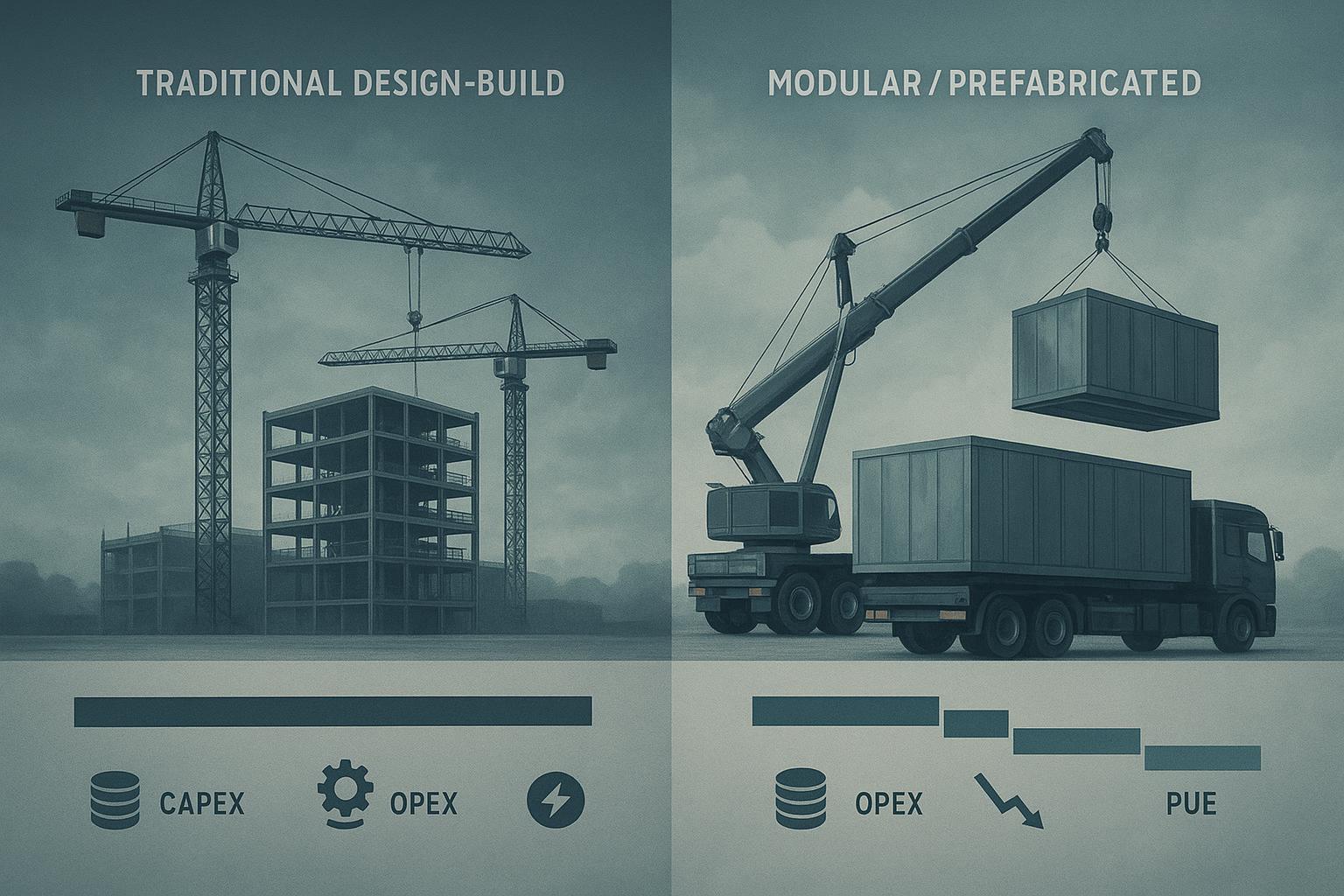
Modular vs. DBB in one page: what actually changes

Modular and traditional DBB differ in three levers that drive economics:

1. Scope and delivery

• Modular: Factory‑built power/cooling modules and plant rooms with standardized interfaces; parallel fabrication and site prep; repeatable QA/commissioning.

• DBB: Custom design, sequential tendering and trades, more on‑site fabrication; longer critical path, higher coordination variability.

2. Cost timing and scale

• Modular: Phased CAPEX with smaller, repeatable blocks. Pay‑as‑you‑grow defers spend until demand materializes, cutting stranded capacity exposure.

• DBB: Larger upfront CAPEX; more assets are installed and financed before utilization ramps.

3. Efficiency and controls

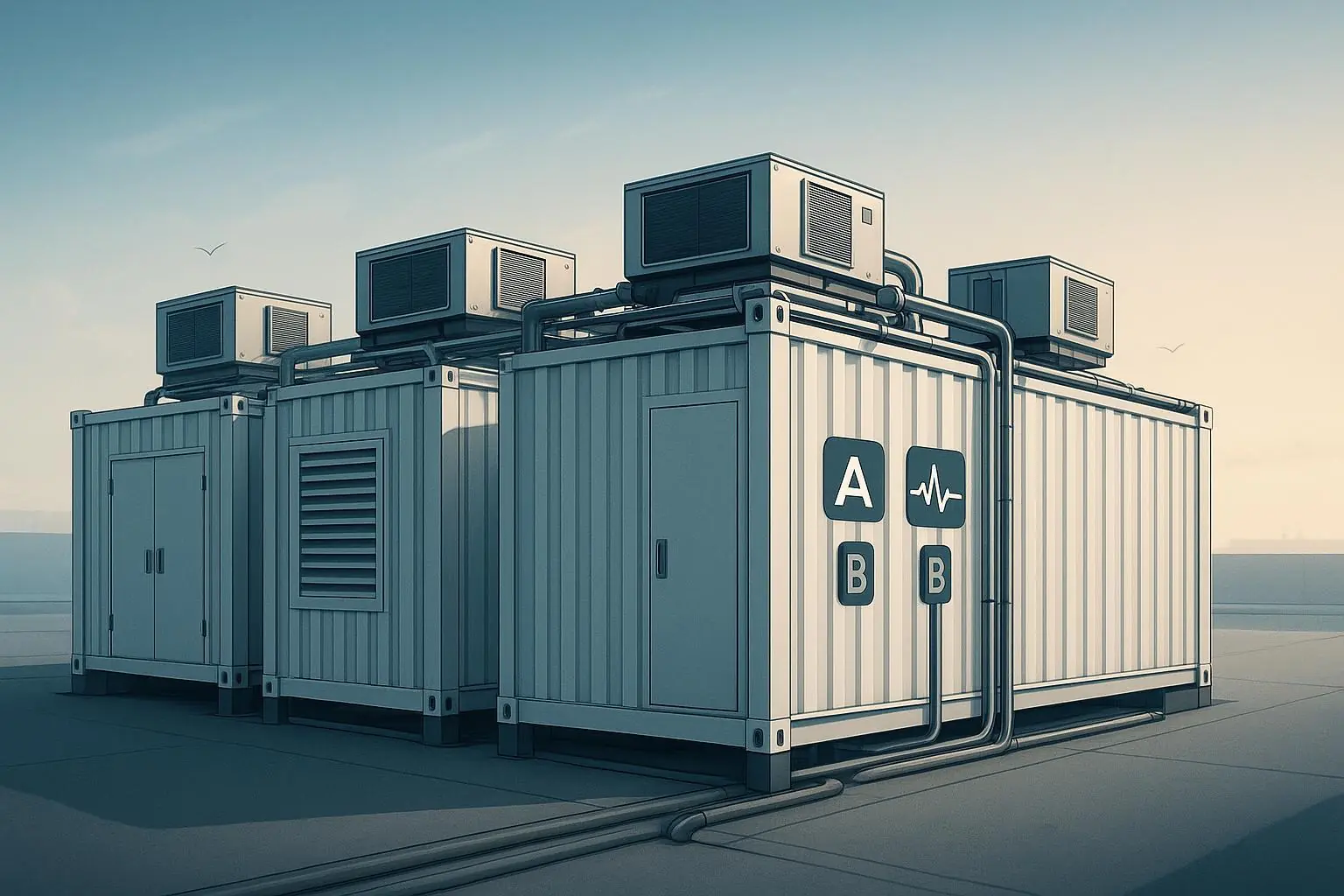
• Modular: Frequently bundles contemporary UPS topologies, variable‑speed drives, economizer‑friendly coil designs, and tighter factory commissioning—enablers of lower PUE. As one example of what “modular UPS scaling” looks like in practice, Coolnet’s UPS power system category illustrates common modular building-block approaches (review any vendor’s specifications against your redundancy and certification requirements).

• DBB: Can achieve equal or better efficiency if engineered deliberately, but retrofit constraints and fragmented commissioning often keep outcomes closer to fleet averages.

Schedule is also different. Industry sources consistently describe modular deployments finishing in months versus 12–24 months for DBB, driven by parallelization and off‑site QA. Treat those ranges as indicative, not guarantees; the meaningful financial question is how many months of interim colocation, delayed revenue, or construction interest you avoid.

For context on typical ranges and trade‑offs (not prescriptive timelines), see comparative guidance from TechTarget’s overview in 2024–2025 and modular construction organizations that outline factory QA benefits. A good primer on when to choose each approach is available in TechTarget’s article, “Modular data center vs. traditional: When to choose each,” which frames schedule and risk at a high level: TechTarget modular vs traditional overview.

PUE fundamentals: why boundaries matter to TCO

Power Usage Effectiveness (PUE) converts engineering choices into energy cost. Measured correctly, it is the ratio of total facility energy to IT equipment energy over the same period.

• Formal definition: PUE = Total data center energy / IT equipment energy, measured on a continuous 12‑month basis with metering boundary classes (PUE0–PUE3) as described in ISO/IEC 30134‑2. Disclose inclusions like UPS losses, fans, pumps, humidification, lighting, and any heat‑recovery auxiliaries. Summaries of the standard and boundary guidance are available from standards libraries and technical explainers, for example the ISO/IEC 30134‑2 synopsis: ISO/IEC 30134‑2 overview and explainers.

• Industry benchmark: The Uptime Institute’s Global Data Center Survey 2024 reports an industry‑average annual PUE of about 1.56, with newer/larger facilities typically achieving materially lower values (≈1.30–1.35 is common for modern builds). See Uptime’s 2024 report and commentary: Uptime Institute 2024 survey report.

Practical implication: If two otherwise comparable designs differ by 0.20–0.25 in PUE, the delta multiplies directly through to annual energy OPEX.

How to model modular data center TCO (step by step)

Start with a five‑ to ten‑year horizon and a linear load ramp. Compare a traditional “build most upfront” baseline to modular phasing. Keep inclusions/exclusions explicit so the comparison stays apples‑to‑apples.

Inclusions typically cover facility CAPEX (power and cooling plant and distribution sized to the capacity under comparison), energy OPEX (electricity for mechanicals and electrical losses), maintenance OPEX (often 2–5% of subsystem CAPEX annually), and commissioning/QA (embedded in modular CAPEX, or itemized for DBB if separate). Exclusions often include land and core shell beyond the MEP scope, financing beyond a simple carry proxy used in schedule examples, and location‑specific taxes or incentives. Document anything you omit.

Core formulas to reuse

• IT energy (kWh/yr) = Average IT kW × 8,760 × utilization

• Facility energy (kWh/yr) = IT energy × PUE

• Energy OPEX ($/yr) = Facility energy × blended electricity price ($/kWh)

• Maintenance OPEX ($/yr) ≈ 2–5% of relevant plant CAPEX

• Simple payback (years) = Incremental CAPEX / Annual savings

• If you need a quick way to sanity-check what vendors include in “precision air conditioning” O&M assumptions (filters, belts, compressors, controls, spares), a manufacturer reference like Coolnet’s Cool-Smart Series Precision Air Conditioning brochure (PDF) can be useful for scoping—treat it as technical background, not an independent benchmark.

Sensitivity mini‑table (1 MW average IT, illustrate tariff/PUE impact)

Rule of thumb: At 1 MW average IT, each 0.10 of PUE shifts ≈0.876 GWh/year. Multiply by your tariff for a quick savings estimate.

Scenario models: turning PUE and phasing into dollars

Assumptions common to all examples

• Linear load growth from 30% to 80% over 5 years

• Electricity price bands applied per region later; base illustration uses a neutral $0.12/kWh

• Maintenance = 3% of plant CAPEX annually (cooling and UPS/distribution)

• Traditional PUE baseline = 1.56; modern/modular PUE target = 1.32 (within the 1.30–1.35 range)

• Module size for phasing: 250 kW blocks with proportionate plant

These examples are models, not measurements. Replace inputs with your site data and tariffs.

A) 250 kW pod (single module) — energy OPEX impact

• Average IT load over Year 1 at 30% utilization: 75 kW

• IT energy: 75 × 8,760 ≈ 657,000 kWh

• Facility energy at PUE 1.56: ≈ 1,025,000 kWh; at PUE 1.32: ≈ 867,000 kWh

• Annual energy savings from lower PUE: ≈ 158,000 kWh

• At $0.12/kWh, Year‑1 savings ≈ $18,960; scale linearly with utilization and tariff

Directionally, even small nodes benefit, but the biggest absolute dollars accrue at scale.

B) 1 MW target load — modular phasing vs. upfront build (simple payback)

Two approaches to reach 1 MW ultimate design target:

• Traditional upfront build: Install plant sized for 1 MW at t0; utilization ramps 30%→80% over 5 years.

• Modular phasing: Deploy four 250 kW modules at t0, t18 months, t36 months, and t54 months in sync with demand.

Illustrative CAPEX and OPEX proxies (round figures for modeling only)

• Plant CAPEX per 250 kW module: $1.8M (power, cooling, integration share); traditional upfront plant for 1 MW: $6.5M due to scale efficiencies but with full carry from day one.

• Maintenance OPEX at 3%/yr of installed plant CAPEX

• PUE: 1.56 for the traditional baseline; 1.32 for the modular build

Energy OPEX comparison at average Year‑3 conditions (assume 55% utilization average by then; Avg IT ≈ 550 kW)

• Traditional facility energy: 550 × 8,760 × 1.56 ≈ 7.52 GWh

• Modular facility energy: 550 × 8,760 × 1.32 ≈ 6.37 GWh

• Annual energy delta ≈ 1.15 GWh → at $0.12/kWh, ≈ $138,000/year

Stranded‑capacity and carry cost proxy

• Traditional upfront CAPEX: $6.5M at t0; modular cumulative CAPEX reaches $7.2M by t54 months (4 × $1.8M), but $3.6M of that is deferred by 36–54 months. If construction interest or hurdle rate proxy is 6%, the deferral reduces carry by order‑of‑magnitude $300k–$500k NPV vs. full upfront, depending on timing.

Simple payback framing for the modular premium or gap

• If modular had a $0.7M higher cumulative CAPEX by year 5 versus traditional (due to packaging costs) but saves ~$138k/year in energy at mid‑ramp plus ~$100k/year in lower maintenance while also avoiding several hundred thousand dollars in carry/colo costs during early years, simple payback would sit in the 3–5 year band—highly sensitive to tariffs and achieved PUE.

Sensitivity checkpoints

• Every +$0.03/kWh in tariff shortens payback by roughly 20–30% at the 1 MW scale for a 0.24 PUE delta.

• A PUE improvement of only 0.15 roughly halves the annual energy savings relative to the 0.24 case.

C) 5 MW direction of travel — why efficiency dominates over time

At 5 MW average IT load (once fully ramped), a 0.20 PUE improvement saves roughly:

• Facility energy delta ≈ 5,000 kW × 8,760 × 0.20 ≈ 8.76 GWh/year

• At $0.12/kWh, ≈ $1.05M/year; at EU industrial rates around €0.18–0.21/kWh, $1.6–$1.9M/year equivalent

At this scale, efficiency and tariff dominate TCO more than modest CAPEX differentials between delivery models.

Regional electricity price bands you should model

Use ranges, not point estimates, and time‑stamp your assumptions. These authoritative sources provide the orientation for 2024–2026 conditions.

• United States (commercial/industrial context): A reasonable modeling band is roughly $0.07–$0.14/kWh across industrial vs. commercial supply, aligned with national statistics and 2024–2025 monthly updates from the U.S. Energy Information Administration. See EIA’s electricity sales, revenue, and average price materials for sectoral context: EIA sectoral price data and updates.

• European Union and United Kingdom: Non‑household prices generally sit higher; a modeling band of €0.16–€0.21/kWh (ex/incl. certain taxes) is consistent with Eurostat 2024 H1–H2 data and UK manufacturing prices recorded in late 2024. See Eurostat’s electricity price statistics and the UK DESNZ Quarterly Energy Prices: Eurostat non‑household electricity price statistics and UK DESNZ QEP December 2024.

• Middle East (UAE, Saudi Arabia): Many industrial tariffs are materially lower than EU/UK levels; modeling bands of roughly $0.05–$0.10/kWh are reasonable starting points for UAE/SA projects, but confirm local slab and surcharge rules. Public materials from DEWA (UAE) and Saudi regulators provide context: DEWA business tariff and fuel surcharge context and Saudi Electricity Company tariff categories.

• Southeast Asia (illustrative): Vietnam’s 2024–2025 guidance implies ~ $0.065–$0.126/kWh industrial bands depending on TOU; Singapore/Malaysia/Thailand often fall in mid‑ to high‑single‑digit cents to low‑teens USD cents per kWh. See EVN/MoIT and national regulator pages for time‑of‑use schedules: Vietnam EVN/MoIT tariff update (2024).

Two quick rules of thumb

• At 1 MW average IT load, every 0.10 change in PUE moves annual energy by ≈ 0.876 GWh, equal to ≈ $88k at $0.10/kWh and ≈ $175k at $0.20/kWh.

• High tariffs (EU/UK) make efficiency gains pay back faster; low tariffs (ME) tilt the balance toward CAPEX and schedule savings.

Table: PUE benchmarks and what to model

Sources: Uptime Institute Global Data Center Survey 2024 (industry average ≈1.56) — see the 2024 survey report for details: Uptime Institute 2024 survey report. PUE definition and boundary guidance: ISO/IEC 30134‑2 explainers.

Pay‑as‑you‑grow economics: stranded capacity and cashflow timing

The main economic win from modular is not a magic discount on equipment; it’s better timing. Here’s the deal: if demand ramps, installing capacity in 250–500 kW stages reduces years of carrying underutilized plant.

Mechanics to quantify

• Stranded capacity avoidance: Compare the area under the curve between installed capacity and actual IT load over time. Every kW‑year of overbuild has a carrying cost (interest, depreciation, maintenance, floor space, auxiliary energy losses).

• Deferred CAPEX: Later modules shift outlays to when revenue or utilization justifies them, improving cashflow and often IRR (even if we focus here on simple payback).

• Schedule effects: Factory parallelization can reduce interim colocation expenses and construction interest months. Instead of promising “6 months faster,” quantify what one, two, or three months saved would be worth at your colo rate or WACC.

Worked mini‑example (1 MW program)

• Traditional: $6.5M upfront at t0; colo bridge cost $120k/month for 6 months while the facility completes = $720k.

• Modular: First 250 kW ready earlier, trimming colo to 3 months for initial workloads = $360k; add two more modules by month 36; the last by month 54.

• Result: $360k avoided colo + energy savings from PUE + maintenance trimmed on not‑yet‑installed plant yields a blended annual savings picture that typically puts simple payback in the low‑single‑digit years if tariffs are moderate‑to‑high and PUE improvement ≥0.20.

Compliance and policy nudges that shift TCO

Regulation doesn’t just add paperwork; it changes what “good” looks like economically.

• EU reporting and ratings: The recast Energy Efficiency Directive (EU/2023/1791) and Delegated Regulation (EU) 2024/1364 require larger data centers to report annual KPIs including PUE, heat‑reuse factors, water metric, and renewable share into an EU database. The European Commission’s explainer outlines scope and timing, with first reports covering 2023 data submitted in 2024 and ongoing annual submissions thereafter. See the Commission’s summary: European Commission energy performance data centres explainer.

• Economic implication: Documented efficiency (lower PUE), readiness for heat reuse, and transparent metering plans reduce compliance risk and may unlock incentives in some jurisdictions or improve community acceptance, indirectly improving TCO by de‑risking approvals and avoiding redesigns.

What to ask for in RFPs and bid packs

• Target and boundary for PUE per ISO/IEC 30134‑2, including metering plan (class, accuracy, aggregation period) and M&V process.

• Phasing plan aligned to your five‑year load forecast (module sizes, commissioning windows, interconnect milestones).

• Regionalized energy OPEX model with tariff bands and sensitivity tables (±25–50%).

• Maintenance assumptions as % of subsystem CAPEX and sparing/SLA provisions.

• Schedule risk register and quantified bridge‑cost scenarios (colo, interest carry).

• Integration plan for future high‑density zones (e.g., liquid‑cooling readiness) without overbuilding today. If you want a concrete taxonomy of liquid-cooling approaches to reference in stakeholder discussions, see Coolnet’s liquid cooling product category as a vendor example.

• Compliance roadmap for local energy reporting and any heat‑reuse or renewable integration.

How to adapt this model to your project

Replace the placeholder electricity price with your contracted rates or TOU‑weighted blends (note taxes and surcharges); set realistic PUE targets based on climate, cooling mode, and controls and confirm the ISO/IEC boundary class; calibrate the load ramp with business roadmaps and test slower/faster ramps to visualize stranded‑capacity impacts; choose module sizes to match UPS/chiller efficiency curves and redundancy rules; run sensitivities at ±0.05 PUE, ±25% tariff, and ±10 percentage points utilization; and document any exclusions (land, grid fees, abnormal groundworks) so comparisons remain fair.

Summary: the shape of the decision

For greenfield builds, modular data center TCO advantages show up in timing and efficiency. Phasing curbs stranded capacity and carries CAPEX forward to when it’s needed; packaging modern plant and QA commonly lands a PUE improvement in the 0.20 range if well executed. In high‑tariff regions, energy savings dominate over time; in low‑tariff contexts, schedule and carry savings matter more. Use the formulas here, disclose boundaries, and pressure‑test assumptions with regional price bands and realistic ramps. If you do, the debate shifts from anecdotes to numbers—and your payback window becomes a planning parameter rather than a guess.