Overcooling is expensive. So is “manual optimization” that works for one season—and quietly breaks in the next.
If you’re responsible for building or expanding an IDC, you’ve probably seen this pattern:
The facility meets inlet temperature limits, but PUE drifts as load and weather change.
Water usage spikes in summer because towers run harder, or because you’re stuck in a conservative set of setpoints.
A retrofit “improvement” looks great on paper—until someone asks whether the comparison was weather-normalized.
This guide is a step-by-step playbook for how AI cooling improves PUE and WUE in practice—and how to measure it in a way that survives compliance review.
Key Takeaway: Treat “AI cooling” as supervisory control that coordinates setpoints, dispatch, and VFD curves under explicit safety constraints—not as a dashboard feature.
Prerequisites (what you need before you optimize anything)
You don’t need a perfect digital twin to start, but you do need clean boundaries and a minimum set of meters.
1) Define measurement boundaries and metering points
You’ll be calculating:
PUE = Total facility energy ÷ IT equipment energy
WUE = Total on-site water use ÷ IT equipment energy
For WUE, use The Green Grid’s formal definition in the Water Usage Effectiveness (WUE) white paper (2011), which uses liters per IT kWh (L/kWh).
For PUE measurement consistency (metering boundaries, levels, and comparison cautions), use the Green Grid’s PUE: A Comprehensive Examination of the Metric (hosted by LBNL).
2) Collect the minimum tag list (you can expand later)
At minimum, you want:
IT energy (kWh) at UPS output or PDU output (pick one method and stick with it)
Total facility energy (kWh) at the utility boundary (or your best equivalent)
Cooling plant electricals: chiller kW, tower fan kW, primary/secondary pump kW, CRAH/CRAC fan kW
Air side: rack inlet temps (multiple heights), supply/return air temps, humidity/dew point (at least representative points)
Water side: CHW supply/return temps, CW supply/return temps (if applicable), flows and/or valve positions
3) Get weather data that matches your site
For water-side systems, wet-bulb temperature matters most; for air-side economization, dry-bulb and humidity constraints matter.
If you don’t have onsite measurements, use a credible nearby station. For basic normalization, degree-day datasets are also usable; the U.S. EIA explains how degree days work.
Step 1 — Compute a baseline PUE and WUE (with explicit assumptions)
Action: Pick a baseline window (e.g., 4–8 weeks) where:
IT load is reasonably stable, or at least well-measured
major maintenance events are excluded
control sequences are unchanged
Worked example: baseline PUE
Assume your baseline month shows:
Total facility energy = 1,200,000 kWh
IT equipment energy = 900,000 kWh
Then:
PUE = 1,200,000 ÷ 900,000 = 1.33
Worked example: baseline WUE (site)
Assume the same month shows:
Cooling + humidification water = 1,800,000 liters
IT equipment energy = 900,000 kWh
Then:
WUE (site) = 1,800,000 ÷ 900,000 = 2.0 L/kWh
Done when: You can reproduce those numbers from your meters, and you can explain the metering point choices in one slide.
Step 2 — Build a weather-normalized PUE (and WUE) baseline
Raw before/after comparisons are often misleading because cooling energy and water use move with weather.
You have two practical options that are defensible without turning this into a research project:
Option A: Wet-bulb binning (recommended for tower/economizer-heavy plants)
Action:
Split hours into wet-bulb bins (for example: 5°F increments).
For each bin, compute:
average cooling plant kW
average tower make-up water
average IT kW
Compare “before” vs “after” inside each bin.
Why it works: You’re controlling for the main environmental driver of tower performance (wet-bulb).
Option B: Degree-day normalization (simple, widely used)
Action:
Compute cooling degree days (CDD) for each period.
Normalize cooling-related kWh by CDD.
If you need a simple reference for why degree days are used in normalization, see LBNL’s discussion in On using degree-days to account for the effects of weather on energy use.
Pro Tip: Normalize by both weather and IT load. If IT kW shifts materially, your cooling energy will shift—even if controls are unchanged.
Done when: You can show that the “after” period improves inside similar weather/load conditions—not only in aggregate.
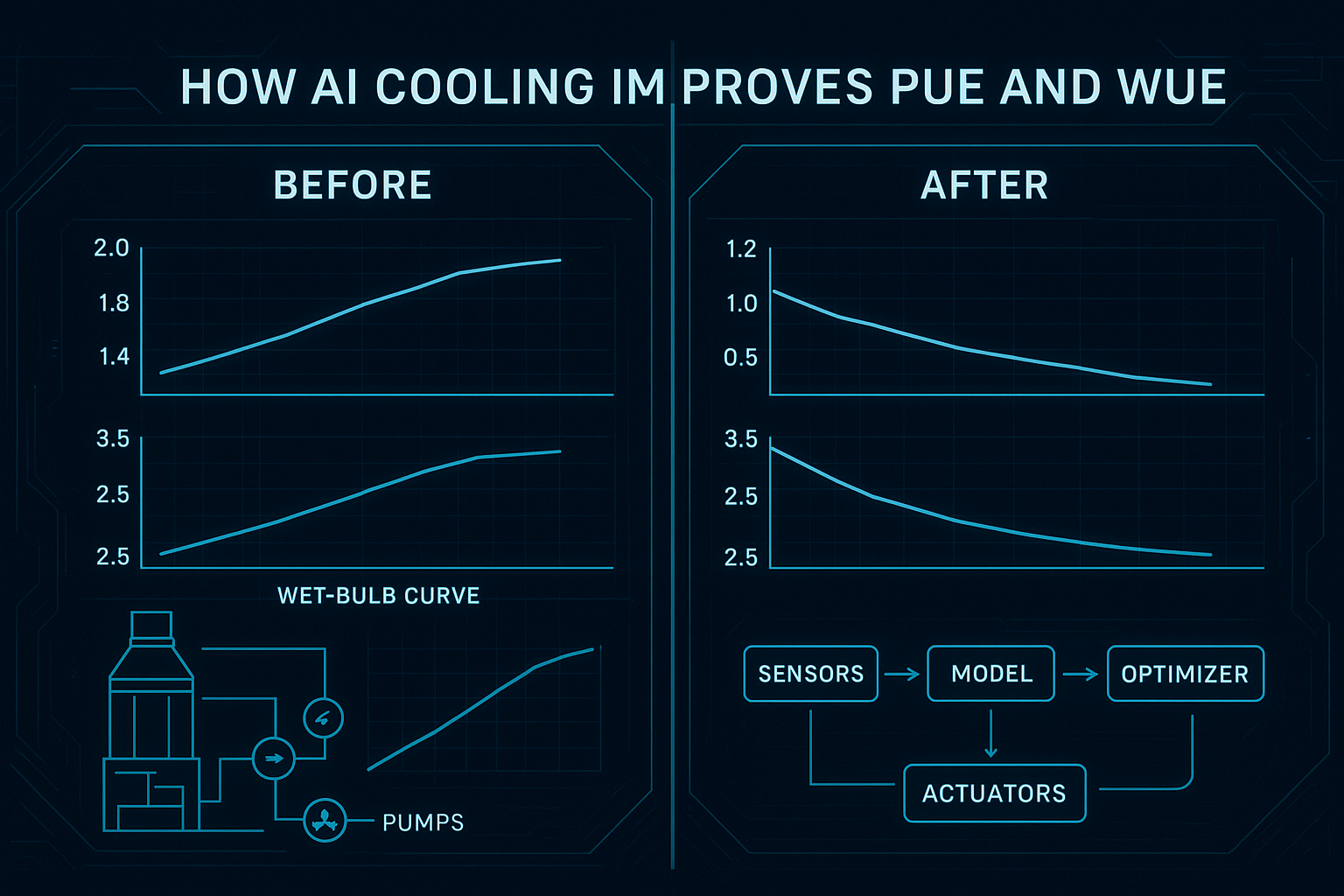
Step 3 — How AI cooling improves PUE and WUE: the three levers
This is where “AI cooling” becomes concrete. The strongest implementations don’t chase one magic setpoint—they reduce control conflicts and safety margins that are bigger than they need to be.
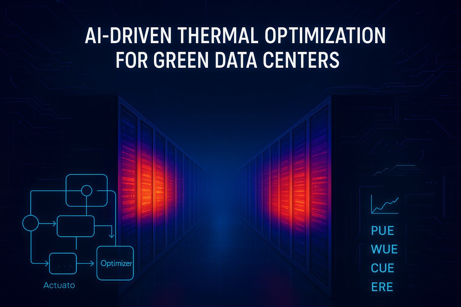
Coolnetpower describes this as closed-loop supervisory control (measure, predict, decide, actuate, verify) in its overview of AI-driven thermal optimization for green data centers.
Lever 1: Data center setpoint optimization (air, water, and hybrid)
What changes:
Supply air temperature targets
Chilled water supply temperature (CHWST)
Condenser water temperature targets (CWST)
Differential pressure setpoints for pumps
In hybrid environments, zone-level heat split between air and liquid
Mechanism (why it improves PUE/WUE):
Many sites run “too cold” because it’s the simplest way to avoid alarms.
Supervisory optimization can safely raise setpoints within constraints, reducing compressor work and often increasing economizer hours.
Constraints you must hard-code:
Rack inlet temperature envelope (aligned to ASHRAE guidance for your equipment class)
Dew point and humidity constraints (to avoid corrosion/ESD risk)
Minimum flow constraints (to protect pumps/heat exchangers)
Rate-of-change limits (to avoid oscillation)
Fallback mode when telemetry is missing or anomalous
⚠️ Warning: A system that can explore without constraints can “learn” the wrong behavior on atypical days (maintenance, partial failures, unusual load).
Lever 2: Waterside economizer + tower dispatch (when to use “free cooling”)
Economizer hours are where energy and water trade-offs show up.
Air-side economizers reduce mechanical cooling, but require careful particulate/humidity control.
A waterside economizer uses tower/ambient conditions to cool via heat exchange and reduce chiller runtime.
ENERGY STAR’s guidance on water-side economizers for data centers is a practical reference for what drives ROI and what makes retrofits harder than they look.
The key dispatch variable: wet-bulb temperature. Cooling towers are fundamentally limited by wet-bulb conditions, not dry-bulb.
A simple operational framing:
If tower + heat exchanger can meet your required chilled water supply temperature, use economizer mode.
If not, stage chillers—but don’t over-punish the towers with unnecessarily low approach targets.
Where AI helps:
Predicts short-horizon changes (weather, load), so it can avoid mode-hunting.
Optimizes the combined energy of chiller + towers + pumps, not one subsystem.
Lever 3: Fan and pump curve optimization (the hidden “big lever”)
Fans and pumps are where small control changes can yield large power differences.
The reason is the affinity law relationship: power scales approximately with the cube of speed. Upsite summarizes this in a data center context in its explainer on fan affinity laws and energy savings.
A practical example:
If you can reduce fan speed from 100% to 80%, power can drop to roughly 0.8³ = 0.512 (about a 49% reduction) while still maintaining acceptable inlet temperatures.
What AI optimizes here:
Static pressure reset / airflow targets (don’t run fans harder than the most constrained zone requires)
Pump differential pressure reset (reduce throttling losses)
Coordination so one loop doesn’t fight another (e.g., fans ramping up because a water setpoint was tightened unnecessarily)
For deeper control detail, the ACEEE paper on static pressure reset control algorithms is a useful reference point for demand-based reset logic.
Step 4 — Implement supervisory optimization safely (and win operator trust)
This is where many projects fail—not technically, but operationally.
Action plan:
Start read-only (2–4 weeks)
Build dashboards and anomaly detection.
Confirm time synchronization and sensor quality.
Pilot one setpoint loop (2–6 weeks)
Example: CHWST reset or CRAH fan speed optimization.
Apply strict rate limits and rollback.
Add dispatch optimization
Economizer/tower vs chiller staging with clear mode logic and anti-hunting.
Expand endpoints gradually
Only after you can demonstrate safety and stable gains.
Done when: Operators can answer “what changed” on any day, and can revert to safe sequences without drama.
Step 5 — Prove it with before/after dashboards (what to show)
Dashboards are not the optimization—but they are how you get sign-off.
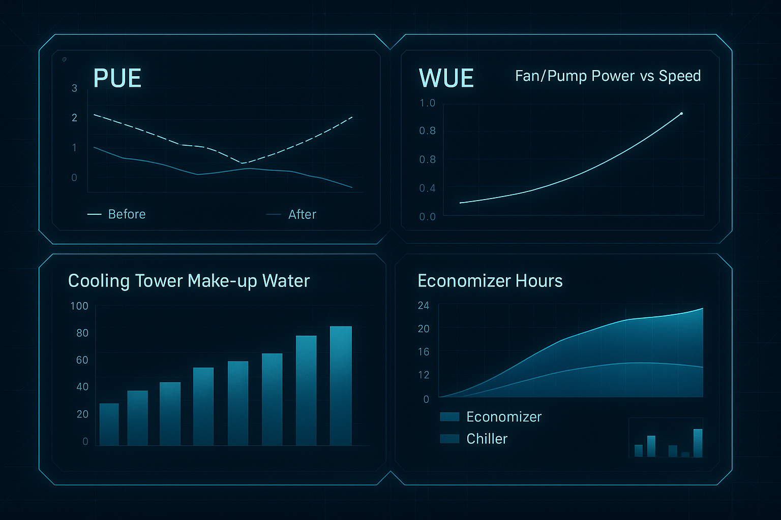
Here’s what a defensible “before vs after” view should include:
PUE trend with the “before” and “after” periods clearly marked
WUE (site) trend, plus tower make-up water (or equivalent)
Economizer hours and mode state (economizer vs mechanical)
Cooling plant power breakdown (chiller, pumps, towers, CRAH/CRAC)
Constraint margins (inlet temperature excursions, dew point margin)
Verification checkpoint (what to document):
Baseline window and optimized window
Normalization method used (wet-bulb bins or degree days)
IT load normalization method used
Any non-routine events (maintenance, partial outages)
Common questions (and the short, practical answers)
Typical PUE delta under similar loads?
It depends on what’s “broken” today. The biggest gains usually come from eliminating overcooling and control conflicts—not from squeezing a single subsystem. For credibility, report results inside weather/load-normalized bins, not as a single headline number.
How is WUE reduced with less tower use?
Primarily by changing dispatch and setpoints so you can:
run towers less aggressively when they’re not needed
increase economizer hours without forcing unnecessary evaporation
shift to higher temperature liquid loops where feasible (reducing compressor hours and sometimes reducing tower demand)
What seasonal/weather impacts are modeled?
At minimum: wet-bulb (tower capability), dry-bulb (air-side economizer potential), and humidity/dew point constraints. Good implementations also include short-horizon forecasts to avoid mode-hunting.
Any trade-offs with reliability or noise?
Yes—if controls aren’t bounded. Aggressive setpoint changes can create instability; higher fan speeds can raise noise. That’s why rate-of-change limits, fallback modes, and clear constraint monitoring are non-negotiable.
How to separate IT vs cooling savings?
Start by separating metering (IT kWh vs cooling plant kWh). Then normalize cooling energy by IT load and weather bins. If you can’t separate meters, be honest about attribution limits.
Where Coolnetpower fits (without turning this into a sales pitch)
If you’re evaluating partners, the practical question isn’t “who has AI?” It’s “who can instrument, integrate, and operate closed-loop control safely?”
Coolnetpower positions AI-driven thermal optimization as supervisory control and describes the closed-loop approach in its article on AI-driven thermal optimization (linked earlier). For solution context across cooling and monitoring layers, see the Coolnetpower solution overview.
Next steps (procurement-friendly)
If you want to scope this as a project, the fastest way to de-risk it is to standardize the inputs.
Request a commissioning checklist + tag list for AI cooling optimization (meters, sensors, naming conventions, and a minimal weather-normalized M&V plan).