Coolnet modular TCO: 5–10 year cost analysis (FAQ) for 200–400 kW pods — modeling modular data center TCO

Modern modular data centers let you add capacity in standardized blocks, but the economics must pencil out over 5–10 years. This FAQ gives a clear, spreadsheet‑ready way to model modular data center TCO for a 200–400 kW pod: itemized CAPEX and install/commissioning, PUE‑driven energy OPEX under regional tariff scenarios, payback/NPV mechanics, financing options (36/60/84 months as structures), and how to treat decommissioning and residual value.

Table of Contents

Key takeaways

Modular data center TCO is the sum of equipment CAPEX, integration and commissioning, energy OPEX driven by PUE, maintenance OPEX, financing cash flows, and end‑of‑life residuals.
Use ISO/IEC 30134‑2 boundaries for PUE, a baseline of ~1.25 for a well‑executed pod at high load, and sensitivity at 1.20/1.30/1.40; document utilization ramps (e.g., 40%→70%→90%).
Annual energy OPEX formula: IT kW × 8,760 × PUE × tariff. Small PUE changes materially shift OPEX; validate at measured loads.
Finance changes the timing (and cost) of cash flows; test capex vs. lease (36/60/84 months) and show payback under multiple tariff paths.
Treat residual and decommissioning explicitly; standard modules can have resale or redeploy value, but confirm with market quotes.

FAQ — modular data center TCO (200–400 kW pods)

What’s included in 5–10 year modular data center TCO for a 200–400 kW pod?

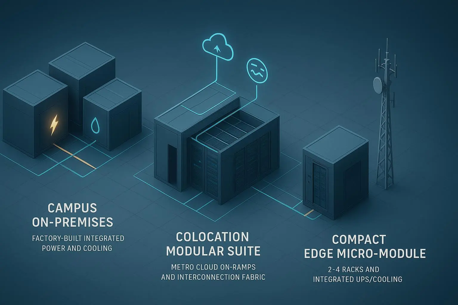
Short answer: Everything you’ll pay from day zero to exit for the pod’s scope. That typically spans equipment (UPS, distribution, racks, row coolers), prefab enclosures or frames, transport, site prep, installation, commissioning, energy and maintenance OPEX, optional financing costs, and decommissioning minus any resale value. Think of TCO as a cashflow story, not just a purchase price.

Scope checklist for a 200–400 kW pod:

Equipment and prefab assemblies; power skids, in‑row cooling, containment, monitoring/BMS, racks, structured cabling interface
Integration, transport, cranage, site prep, installation labor, and commissioning (FAT/SAT/IST)
Energy OPEX (PUE‑driven), maintenance OPEX (service contracts, spares), taxes/permits as applicable
Financing (if used): origination, interest, lease payments; insurance where required
End‑of‑life: decommissioning, recycling, and any salvage/resale

How do I itemize CAPEX, installation, and commissioning?

Break equipment CAPEX by system (UPS/PDUs/busway, row coolers, containment, racks, sensors/BMS, prefab structure). Then add integration/installation: transport and rigging, electrical/mechanical tie‑ins, controls integration, and test equipment rentals. Commissioning costs cover factory acceptance (where applicable), site acceptance, integrated systems testing (IST), and corrective punch‑list work. Many teams also budget for spares and O&M toolkits at day one.

Tip: Prefabrication can compress install time and reduce schedule risk. It doesn’t remove commissioning; it focuses it on interfaces and IST quality.

What PUE boundary should I use, and what’s a realistic baseline?

Use the ISO/IEC 30134‑2 definition of Power Usage Effectiveness and state your measurement boundary and category up front. In short: PUE = total facility energy / IT equipment energy, ideally measured over a continuous 12‑month period with appropriate metering at or near the IT boundary. See the ISO catalog overview of the standard and public explainers for boundary categories in the 2026 listing and 2024 summaries via the ISO portal and Sunbird/DCIM practitioners.

Reference: ISO/IEC 30134‑2 boundary guidance in the 2026 catalog and the ISO overview pages: see the descriptive summary in the ISO/IEC 30134‑2 catalog and overview (2026/portal) and ISO’s 30134‑2 standard page.
Context: Industry surveys place the global average PUE near the mid‑1.5s, with newer/larger sites often reporting ~1.3 or better at high load. See Uptime Institute’s 2024 survey reporting.

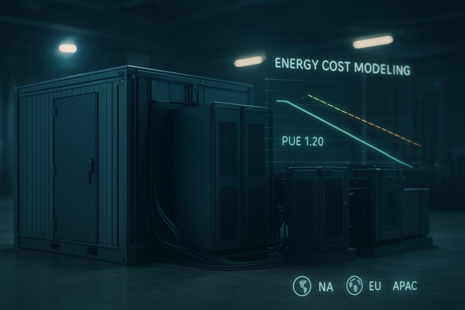
For a well‑designed 200–400 kW pod operating at high utilization, a baseline PUE of ~1.25 is reasonable with sensitivity bands at 1.20, 1.30, and 1.40. At part‑load, expect some PUE degradation; document your actual readings.

How do I calculate annual energy OPEX?

Use this core equation and keep every unit explicit.

Annual energy OPEX ($/yr) = IT_Load(kW) × 8,760(hr/yr) × PUE × Tariff($/kWh)

Example (illustrative): 300 kW average IT load, PUE 1.25, tariff $0.10/kWh → 300 × 8,760 × 1.25 × $0.10 ≈ $328,500 per year. A 0.05 PUE improvement (~4%) lowers this by roughly $13,000/yr at the same load and tariff. That’s why metering accuracy and thermal optimization matter.

For methodology context on modeling and distributions, see the LBNL 2024 United States Data Center Energy Usage Report.

Which electricity price scenarios should I use for North America, Europe, and APAC?

Anchor your ranges to official statistics and then substitute your local large‑user tariffs.

North America: Use U.S. EIA industrial price series and, where relevant, utility‑specific large‑user schedules. Start from the EIA electricity sales/revenue/price portal and extract current industrial ¢/kWh for your state or ISO region: EIA electricity sales, revenue, and price portal.
Europe: Use Eurostat’s non‑household electricity price statistics (size bands available; exclude recoverable taxes to compare) and then adjust for your contract: Eurostat electricity price statistics for non‑households.
APAC: Pull country‑specific regulator data (e.g., Australia AER/ABS, Japan METI/ANRE, Korea KEPCO). Document currency and year and convert to $/kWh consistently.

Model a baseline band per region and test low/medium/high to reflect contract variability.

How does a utilization ramp affect PUE and energy OPEX?

Two effects stack: at lower load, fixed losses dominate so PUE tends to rise; and your IT kWh are simply lower. A realistic ramp might average 40% in year 1, 70% in year 2, 90% in steady state. Record measured PUE per stage if you can. If not, keep a sensitivity (e.g., 1.30 at 40%, 1.25 at 70%, 1.22–1.25 at 90%) based on your design and climate. Here’s the deal: even a small PUE improvement at high load pays more annually than a larger improvement at very low load.

What does a simple 5‑ and 10‑year payback look like under different tariffs?

Illustrative outline (substitute your numbers):

Record upfront CAPEX + install/commissioning.
Compute annual energy OPEX for each year with your utilization and PUE assumptions.
Add maintenance OPEX.
If financing, replace the upfront CAPEX with lease/loan payments and fees.
Sum cumulative net cashflow; simple payback is the year cumulative savings vs. a baseline alternative turn positive.

Worked example (illustrative only):

Baseline choice: stick‑built alternative OPEX assumed at PUE 1.35; modular pod at PUE 1.25.
IT average: 300 kW; tariff: $0.10/kWh; utilization ramps 40%→70%→90% (apply to IT load); hold PUE per stage as above.
Annual energy savings vs. baseline at 90% load ≈ 300 × 8,760 × (1.35–1.25) × $0.10 ≈ $26,280.
Over 10 years (steady portion), that’s ~$260k before escalation. Discount to present value to compare to your CAPEX delta.

For market context on deployment and cost drivers (not a terms guide), see CBRE’s North America Data Center Trends H2 2024.

What maintenance OPEX should I plan for?

Plan for preventive maintenance of UPS/power distribution, row coolers, controls/BMS, and periodic IST drills. Include consumables (filters), spares, and emergency response provisions. Public, standardized $/kW‑year ranges vary widely and weren’t identified in citable 2024–2026 sources; many teams model maintenance as a negotiated service contract informed by equipment count and duty cycles. The most reliable input is your vendor and service‑partner quote; treat it as a separate line from energy OPEX.

What commissioning activities (FAT/SAT/IST) add cost and schedule risk?

Expect three layers, scaled to your pod:

FAT: factory acceptance at the module or subsystem level (where applicable).
SAT: site acceptance for installed equipment and controls integration.
IST: integrated systems testing with load banks, failure scenarios, alarms, and run‑time validation.

Budget for test rentals, controls tuning, punch‑list corrections, and retests. Prefab helps, but commissioning rigor is non‑negotiable for reliability.

How do financing or leasing terms (36/60/84 months) change cash flow and NPV?

Financing converts a lump‑sum CAPEX into periodic payments and fees, changing both timing and total cost. Common structures include equipment loans, capital or FMV leases, and project‑style facilities for larger campuses. Tenors like 36/60/84 months are typical for equipment finance; effective rates depend on credit, asset life, and residual treatment. Compare:

Cash purchase: upfront CAPEX; lower total financing cost; opportunity cost equals your internal WACC.
Lease/loan: spreads cost; increases nominal outlay with interest; may speed time‑to‑value if capacity is urgently needed.

Always model NPV/IRR with your discount rate, taxes, and any residual/buyout terms. Public program examples for broader context include the U.S. SBA 504 long‑tenor loan overview (not data‑center‑specific) and general equipment finance primers (use lender quotes for actual terms).

How do I treat decommissioning and residual or salvage value?

State an explicit assumption for year‑5 or year‑10 residual, and separate it from decommissioning costs. Standardized modules can be re‑deployed, resold, or harvested for components (UPS frames, in‑row coolers, racks). Salvage depends on condition, demand, and logistics. Use market quotes or recent resale comps; avoid assuming aggressive residuals without evidence. If your lessor sets an FMV residual, use that figure in your lease NPV math.

How do prefab ratios and phased buildouts affect cash flow vs. stick‑built projects?

Pods shift spend from bespoke construction to manufactured assemblies. Benefits often include shorter schedule, parallel off‑site fabrication, and right‑sizing capacity to demand (pay‑as‑you‑grow). Cash flows are staged in smaller increments (200–400 kW at a time), which can reduce carrying costs for underutilized capacity early in the program.

Where do row cooling and free cooling fit into the model?

Row‑based precision cooling usually serves as the pod’s thermal backbone; consider aisle containment and controls integration to steady PUE across the load range. In suitable climates, economizer or free‑cooling modes can drive seasonal PUE improvements. For form‑factor context on row cooling, see the in‑row category page here: precision in‑row cooling systems and an overview of free‑cooling options.

Where can I see a representative module form factor for a 200–400 kW scope?

For a sense of how a prefabricated pod integrates racks, power, and in‑row cooling with containment and monitoring, review a modular solution example like the MetaRow modular data center solution for scalable infrastructure. As a neutral reference point, vendors such as Coolnet support modular architectures that can be applied in greenfield “starter pod” deployments; specific pricing and financing should be obtained via formal quotes.

Scenario table — PUE and tariff sensitivity (illustrative math)

The table shows how to compute annual facility energy and OPEX per kW of average IT load under common PUE values. Replace the tariff column with your local $/kWh.

PUE	Facility kWh per kW IT (per year)	OPEX per kW IT at $0.08/kWh	OPEX per kW IT at $0.12/kWh
1.20	8,760 × 1.20 = 10,512	$840.96	$1,261.44
1.25	8,760 × 1.25 = 10,950	$876.00	$1,314.00
1.30	8,760 × 1.30 = 11,388	$911.04	$1,366.56
1.40	8,760 × 1.40 = 12,264	$981.12	$1,471.68

Notes:

Multiply the “per‑kW IT” OPEX above by your average IT kW to get annual $/yr. For a 300 kW pod at PUE 1.25 and $0.12/kWh → 300 × $1,314 ≈ $394,200/yr.
Regional tariff anchors: use the EIA industrial price portal for U.S. data and Eurostat’s non‑household series for EU comparables; for APAC, cite national regulators. Keep unit conversions consistent.