Precision cooling decisions (airflow control, fan technology, economizer strategy, controls, and serviceability) often show up in two places procurement cares about:
Annualized PUE (how much non-IT overhead power you carry year-round)
Five-year TCO (capex + energy + O&M + risk-adjusted service costs)
If you’re building a model, the decision becomes easier when you separate where the savings come from (e.g., reduced fan power, fewer mechanical cooling hours) from what you’re buying (equipment, integration, commissioning, service).
This how-to guide gives you a neutral, five-year model you can use to compare options such as EC fans vs fixed-speed, economizers/free cooling, and the O&M / warranty / incentive levers that typically dominate payback.
Key Takeaway: For a fixed IT energy baseline, a PUE improvement of ΔPUE translates directly into annual kWh savings: ΔkWh ≈ E_IT × ΔPUE. The model is about turning that relationship into a defensible 5-year business case.
Table of Contents
ToggleWhat you’ll build in this five-year data center cooling TCO model
Outputs (what your model should produce):
Baseline vs improved annual facility energy (kWh) and energy cost ($)
Five-year cash flow view (simple payback, optional NPV)
A comparison table for the major cooling options you’re evaluating
Sensitivity charts that show which assumptions drive the result
Scope note: The example numbers and charts below are illustrative. They are not a promise of performance for any specific site.
Step 0 — Gather inputs and set boundaries (don’t skip this)
Before you model anything, decide two things:
Metering boundary for PUE (what “total facility energy” includes)
Which PUE you’re modeling (annualized vs peak)
A practical rule: use annualized PUE when you’re estimating five-year cost. Raritan summarizes why annualized PUE is the metric that captures seasonal variation, while peak PUE describes worst-case conditions and infrastructure sizing in “Comparing Annualized and Peak PUE”.
Also record: redundancy mode (N, N+1, 2N), supply/return temperature targets, humidity/dew-point control strategy, and whether the comparison is brownfield retrofit or greenfield design.
Step 1 — Translate PUE into annual energy cost
Use the standard definition:
PUE = Total Facility Energy / IT Equipment Energy
Let:
E_IT = annual IT energy (kWh/year)
PUE = annualized PUE
c_e = electricity price ($/kWh)
Then:
Annual facility energy: E_fac = E_IT × PUE
Annual overhead energy: E_ovh = E_IT × (PUE − 1)
If your goal is to value a PUE improvement from PUE₀ to PUE₁:
Annual kWh saved: ΔE = E_IT × (PUE₀ − PUE₁)
Annual $ saved: Δ$ = ΔE × c_e
This is the simplest way to keep the model honest: if you claim a PUE delta, it must reconcile to annual kWh.
Step 2 — Model the EC fan retrofit energy savings lever (EC vs fixed-speed)
EC fans matter in a five-year model for two reasons:
Efficiency at part load: data halls rarely operate at one steady state; fan power reduction can be meaningful when you can safely reduce airflow.
Control and integration: the economic value often depends on whether your controls and airflow management let you actually run at lower fan speeds.
A practical, model-friendly structure is:
Baseline fan power (kW) and annual runtime (hours)
Expected fan power reduction factor (based on speed reduction + efficiency improvement)
Any added capex (retrofit kit, controls upgrade) and any O&M change
KW Engineering’s retrofit discussion is useful here because it separates two mechanisms—airflow reduction and fan/motor efficiency—in “EC Plug Fan Retrofits”. Treat any savings percentages as site-specific; what you need for the model is the mechanism and a way to test sensitivity.
Step 3 — Model the data center economizer free cooling lever (hours matter more than slogans)
Economizers improve annualized PUE by reducing compressor/chiller hours when outdoor conditions can do part (or all) of the heat rejection work.
Two common categories:
Air-side economizer: uses outside air directly
Water-side economizer: uses cooling towers/dry coolers/heat exchangers to deliver “free cooling” on the water side
For modeling, the key variable is eligible hours under your allowable envelope (temperature + humidity/dew point + air quality constraints).
ENERGY STAR provides a clear, neutral reference point for “ideal conditions” and climate-hour framing in “Use an Air-Side Economizer” and calls out humidity as a first-order constraint.
⚠️ Warning: Don’t model economizer savings as if cooling becomes “free.” Fans, pumps, filtration pressure drop, and control overhead still consume energy—and risk constraints can reduce usable hours.
Step 4 — Add O&M and spares as a first-class term (not a footnote)
In five-year comparisons, O&M differences often come from operational realities rather than headline efficiency:
Filters and filtration management
Rotating components (belts/bearings vs direct-drive plug fans)
Controls maintenance and periodic re-commissioning
Redundancy testing and failover validation
Spares strategy and lead times (controls boards, fan motors, valves)
If you don’t have credible site data, it’s better to be neutral and run sensitivity than to invent a precise annual O&M number.
Step 5 — Treat warranty and service terms as risk-adjusted cost
For mission-critical cooling, warranty and serviceability affect TCO mainly through:
Conditions that preserve coverage (authorized service, documented maintenance)
Startup/commissioning requirements
Response SLA and parts logistics
Vertiv explicitly warns that untrained service on advanced controls can void warranty in its precision cooling maintenance material “Data Center Precision Cooling” (PDF).
In the model, you can represent this as either:
a service contract line item ($/year), or
a risk contingency ($/year) tied to response time and spares availability
Step 6 — Apply incentives and PUE improvement payback rules (US)
US utility programs often support data center efficiency measures (EC motors, VFDs, economizers, controls optimization) via prescriptive or custom incentives.
A concrete example is SRP’s data center rebate fact sheet “SRP Business Solutions — Data Centers” (PDF), which illustrates kWh-based custom incentives and prescriptive measures.
Model incentives conservatively:
subtract incentives from net installed cost (capex)
reflect timing (some programs pay post-verification)
avoid counting the same kWh savings twice if measures interact
Step 7 — Build a five-year view (simple, then robust)
Start with a clear baseline and one improved case.
Illustrative assumptions used for the charts below:
Parameter | Illustrative value |
|---|---|
Annual IT energy (E_IT) | 10,000,000 kWh/year |
Baseline → improved annualized PUE | 1.50 → 1.35 |
Electricity price range | $0.08–$0.20/kWh |
Net upfront cost (capex − incentive) | $525,000 |
O&M delta | $0/year |
Then compute:
Annual savings: E_IT × ΔPUE × c_e
Five-year net benefit (simple): 5 × annual savings − net upfront cost
If you need a procurement-grade model, add discounting (NPV) and rate escalation—but keep the simple version visible for sanity checks.
Step 8 — Sensitivity analysis (what actually drives the answer)
Two visualizations are usually enough to keep the discussion grounded.
1) Tornado chart: sensitivity of five-year net benefit
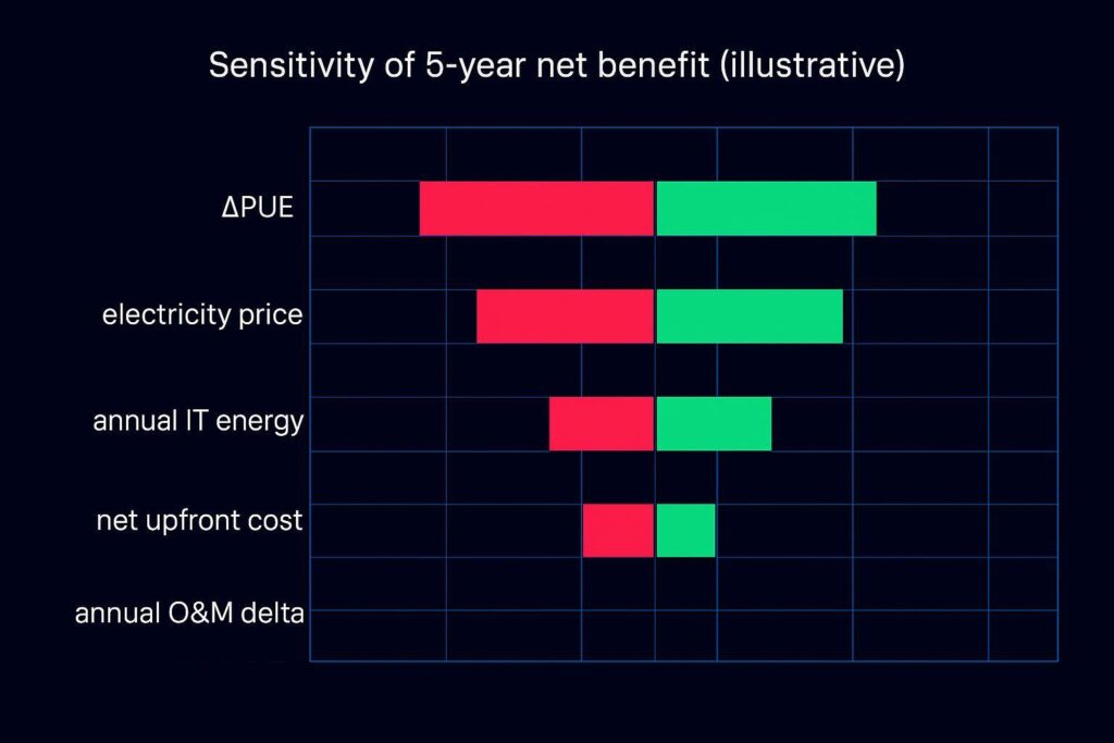
Interpretation:
If ΔPUE is uncertain, it often dominates the spread.
Electricity price is usually the next largest driver.
“Net upfront cost” matters, but it’s often easier to bound than ΔPUE.
2) Payback vs electricity price
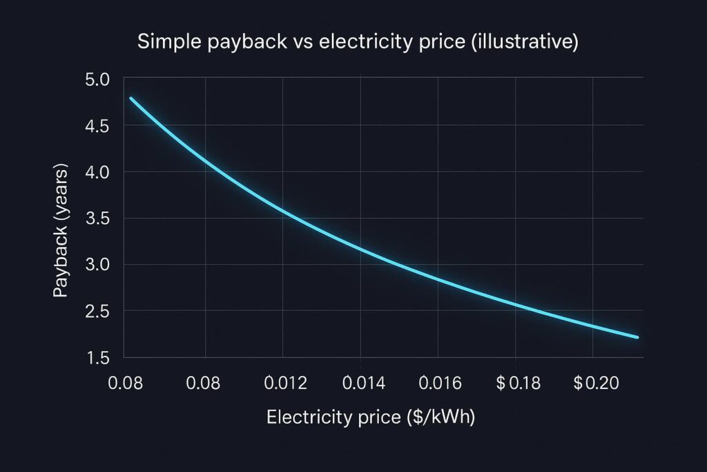
This chart is useful when stakeholders argue about tariffs: it shows how fast payback changes as electricity price moves.
A comparison table you can reuse (EC fans, economizers, O&M, warranties, incentives)
Use this as a neutral “one page” to structure internal discussions.
Lever | Primary impact on PUE | Primary impact on 5-year TCO | What to validate on your site |
|---|---|---|---|
EC fans vs fixed-speed | Reduces fan energy; can enable lower airflow at part load | Energy savings; sometimes lower maintenance (beltless); potential controls cost | Fan power curve, controllability, airflow management maturity |
Economizer / free cooling | Reduces compressor/chiller energy during eligible hours | Energy savings; may add controls/O&M complexity | Eligible hours (dry-bulb + dew point), filtration/air quality, mode-change controls |
O&M program maturity | Indirect (keeps systems near design efficiency) | Can dominate lifecycle cost if PM and spares are weak | PM plan, spares strategy, staffing, recommissioning cadence |
Warranty + service terms | Indirect (reduces downtime and “hidden” cost) | Converts failure risk into predictable service cost | Coverage conditions, SLA, authorized service rules, spare-part logistics |
Incentives | No direct PUE effect | Reduces net capex and payback time | Pre-approval rules, measurement & verification requirements |
Five-year TCO data center cooling: what to include (checklist)
When you pressure-test the model with procurement and ops, confirm you’ve captured:
One-time costs: equipment, installation, controls integration, commissioning, M&V
Recurring costs: energy, planned PM labor, spares replenishment, service contract
“Hard-to-ignore” constraints: redundancy mode, humidity/dew point envelope, air quality / filtration, water usage (if applicable)
Interaction effects: airflow changes influencing economizer hours; setpoint changes influencing eligible hours
Precision cooling vs comfort cooling: what changes in the model
“Comfort cooling” assumptions often break in data halls because the load is high-sensible, continuous, and uptime-driven. In a data center cooling TCO model, the practical differences usually show up as:
Control + part-load behavior (fan modulation, coordination with containment and setpoints)
Reliability and redundancy expectations (failover behavior is part of the requirement)
O&M discipline (spares, alarms, re-commissioning)
You don’t have to argue which category is “better” in general; you just need to model where the cash flows and risks diverge.
Common modeling mistakes (and how to avoid them)
Using peak PUE to justify annual savings: use annualized energy for cost.
Counting economizer hours without humidity/dew point constraints: eligible hours can collapse quickly.
Assuming airflow reduction is “free”: validate with containment, pressure management, and temperature at the IT inlet.
Ignoring maintenance and spares: five-year outcomes often hinge on O&M execution.
Next steps
If you want to apply this model to a real facility, start by making the baseline defensible:
confirm metering boundary and annualized PUE method
capture fan power and cooling plant power over representative seasons
document control sequences and redundancy modes
For an internal selection workflow, you can also use Coolnetpower’s decision framing on CRAC/CRAH vs in-row in Coolnetpower’s decision tree guide, and the emphasis on before/after validation and assumptions in Coolnetpower’s PUE validation FAQ.
CTA: If you’d like, request a commissioning + measurement checklist to validate ΔPUE and avoid model-driven surprises during acceptance.