Validating ROI for a direct-to-chip liquid cooling retrofit is rarely an “energy math” problem. It’s a measurement boundary problem.
If you can’t answer (in writing) what you measured, how you adjusted for weather and load growth, and who signs off on baseline changes, the ROI conversation turns into a dispute.
This guide gives you a 12‑month, audit-ready workflow—built around IPMVP Option B/C framing—so you can validate savings in a way procurement, operations, and finance can all defend.
Key Takeaway: ROI is easiest to defend when you treat commissioning + measurement as one program: define the boundary, instrument it, lock the adjustment rules, then run monthly true‑ups.
Table of Contents
TogglePrerequisites (what you need before you start)
You don’t need perfect instrumentation on day one, but you do need agreement on the basics.
Inputs you should have available (or be able to create in 2–4 weeks):
12 months of baseline data (utility bills, submeter data, or both)
A clear scope statement: which racks/loops are converting to liquid
A commissioning plan and acceptance criteria (leak tests, failover, alarms)
Access to routine independent variables:
outside air temperature / CDD (weather)
IT load (kW and/or kWh) and major configuration changes
Agreement on the M&V approach (Option B, Option C, or hybrid)
If you want a ready-to-use worksheet pack, you can link your internal stakeholders to the downloadable calculator (we’ll reference it again in the Next steps section).
Step 1 — Define the ROI question (and the acceptance threshold)
Input: Your business case (CapEx/OpEx), decision deadline, and what “success” means.
Action: Write the ROI question as a measurable statement:
“We will validate that the liquid cooling retrofit reduces cooling-system kWh per delivered IT kWh by X% (weather- and load-normalized) within 12 months, without increasing unplanned downtime.”
Set an acceptance threshold that matches procurement reality:
payback within a maximum time (e.g., 24–36 months) and
a 12‑month validation milestone (e.g., evidence of trend + verified measurement system)
Output: A 1‑page ROI validation objective (what’s in / what’s out).
Done when: Procurement, facilities, and IT operations agree on (1) the metric, (2) the boundary, and (3) the time window.
Step 2 — Choose your M&V boundary (IPMVP Option B vs Option C)
Input: A one-line retrofit scope and what meters/sensors exist.
Action: Pick the boundary that reduces argument risk.
According to EVO’s IPMVP protocol overview, Option B isolates the retrofit boundary and measures all parameters; Option C looks at whole-facility (or whole subfacility) energy.
In liquid cooling retrofits, the cleanest approach is often a hybrid:
Option B (retrofit isolation) for the liquid loop boundary (CDU + pumps + heat exchanger + controls)
Option C (whole facility/subfacility) to validate that savings are visible at the meter once adjustments are applied
Pro Tip: For auditability, write down the independent variables you’ll use on Day 1 (weather + IT load) and keep them consistent for the full reporting year.
Output: An M&V boundary diagram (even a simple block diagram) and a list of meters/sensors inside the boundary.
Done when: You can point to a single diagram and say: “Savings are calculated inside this box; adjustments are applied using these variables; the whole-meter view is used as a reasonableness check.”
Step 3 — Build the baseline (and document what can change)
Input: 12 months of pre-retrofit data + operating notes.
Action: Define three baseline layers:
Energy baseline period (typical: 12 months)
Operational baseline (setpoints, availability targets, control sequences)
Asset baseline (what equipment existed and how it was configured)
Then classify baseline changes up front:
Routine adjustments (expected, modelable): weather, normal seasonal variation
Non-routine adjustments (NRAs) (discrete events): added racks, major load density shifts, changes in redundancy mode, new cooling equipment, changed setpoints outside agreed bounds
If you’re building Option C models, plan to treat IT load growth as either:
an independent variable in your regression model (routine), or
a non-routine event requiring a documented baseline adjustment (NRA)
Output: A baseline pack (data + assumptions + change log template).
Done when: You have one file that shows baseline period, data sources, and an agreed rule: “These changes trigger an NRA review.”
Worksheet A — Baseline pack template
Item | What to record | Where it comes from |
|---|---|---|
Baseline dates | Start/end; exclude anomalies with justification | Utility/submeter exports |
Weather source | Station + degree-day method | Weather service / degree days tool |
IT load proxy | IT kW / IT kWh / rack count (pick primary) | PDU/UPS/DCIM |
Setpoints | supply temps, approach temps, alarm thresholds | BMS / controls |
Static factors | redundancy mode, operating hours, occupancy limits | Ops runbooks |
Change log | expansions, reconfigurations, maintenance events | Change tickets |
Step 4 — Decide how you’ll normalize for weather (weather normalization)
Input: Weather data choice and metering granularity (monthly vs interval).
Action: Use a regression-based normalization method when weather can materially influence cooling energy (economizers, dry coolers, condenser water temps).
A common baseline regression form is:
E = b*days + h*HDD + c*CDD
Rather than guessing base temperatures, tools can test many bases and select the best fit. Degree Days.net’s baseline regression guidance describes model quality checks such as cross-validated R² and CVRMSE, and flags negative coefficients as a warning sign.
Output: A declared normalization method (degree-day regression or temperature regression) + acceptance criteria for model quality.
Done when: You can compute an adjusted baseline for any month in the reporting period using the same method.
Worksheet B — Weather normalization checklist
Choose weather station and document it
Select model form (CDD-only, HDD-only, or combined)
Choose base temperatures via regression shortlist
Record model coefficients and fit statistics
Define what triggers a model refit (e.g., major operating change)
Step 5 — Normalize for load growth (the part that breaks most ROI claims)
Input: Your IT load measurement plan.
Action: Pick a single “source of truth” variable for IT activity and stick to it.
Recommended hierarchy:
IT kW / IT kWh (metered)
UPS output kW (metered)
PDU/rack count proxies (least preferred; document limitations)
In Option C, treat load growth as either:
a regression variable (routine), or
a non-routine adjustment (NRA) when growth exceeds a pre-agreed threshold (e.g., a step change from a new AI cluster)
Output: A load-normalization rule and threshold.
Done when: Finance can see how you avoid “saving disputes” when IT load rises.
Worksheet C — Independent variables (Option C model)
Variable | Why it matters | Data source | Frequency |
|---|---|---|---|
IT kW (avg/peak) | primary driver of heat load | PDUs/UPS/DCIM | 15-min / hourly |
IT kWh | captures utilization changes | PDUs/UPS/DCIM | daily / monthly |
CDD (or OAT) | affects economizer/compressor hours | weather dataset | daily / monthly |
Setpoint band | shifts cooling energy and risk | BMS/controls | hourly |
Step 6 — Instrument the boundary (minimum viable metering for Option B)
Input: Boundary diagram from Step 2.
Action: For Option B, your rule is simple: measure all parameters needed to compute energy use and verify performance.
At a minimum, plan to capture:
CDU power (kW/kWh) and pump status
supply/return temperatures on the liquid loop
flow rate (per loop or per rack group)
differential pressure (to detect restrictions/leaks)
leak detection and alarm status
For a practical retrofit commissioning + sensor blueprint, Coolnetpower’s direct-to-chip liquid cooling 20–40 kW guide describes leak-test and instrumentation elements you can adapt into your acceptance plan.
Output: Meter list + sensor list + data retention plan.
Done when: You can explain, for any month, which meters produced which savings numbers.
Step 7 — Commission for “M&V readiness,” not just thermal stability
Input: Commissioning schedule and outage windows.
Action: Commissioning is the first place ROI gets proved or lost. If leak alarms chatter, sensors drift, or failover isn’t tested, you’ll spend the year arguing about data.
Build your commissioning plan around evidence:
Pre‑install verification (materials, cleanliness, fluid chemistry assumptions)
Leak and integrity testing (pressure-decay; high-sensitivity detection where appropriate)
Flushing/filtration and cleanliness verification
Functional performance tests
flow balancing to tolerance
sensor calibration
alarm thresholds + interlocks tested
CDU pump failover tested
Thermal soak test (24–72 hours at target load)
Output: A commissioning dossier: test results + sign-offs + “as-built” diagrams.
Done when: You can hand a third party the dossier and they can reproduce your boundary and data sources.
Worksheet D — Commissioning timeline (typical) and deliverables
Time window | What happens | Evidence you should capture |
|---|---|---|
Weeks 0–4 | design finalization, instrumentation plan, outage planning | boundary diagram; meter list; baseline pack |
Weeks 4–8 | install + tie-ins + initial leak/integrity testing | test reports; as-built updates |
Weeks 8–12 | functional tests + failover + thermal soak | acceptance checklist; alarms verified |
Months 3–6 | stabilization + tuning + first true-ups | monthly M&V reports; model validation |
Months 6–12 | steady reporting + NRAs as needed | quarterly executive summaries; dispute log |
Step 8 — Calculate savings monthly (and run a quarterly “audit-grade” true-up)
Input: Meter data + weather + IT load + change log.
Action: Establish a cadence:
Monthly: compute savings and document adjustments
Quarterly: perform a formal true-up (review models, verify data completeness, review NRAs)
Make the savings equation explicit.
Option B (simplified) savings logic
Savings = (baseline liquid-loop energy under equivalent conditions) − (measured liquid-loop energy)
Option C (simplified) savings logic
Adjusted baseline = baseline regression model evaluated at reporting-period weather/load
Savings = adjusted baseline − actual metered energy
Output: Monthly M&V memo + quarterly true-up packet.
Done when: Your savings number can be traced back to raw data, model coefficients, and documented adjustments.
Worksheet E — Monthly M&V memo template (one page)
Section | What to include |
|---|---|
Boundary | what’s included/excluded |
Data completeness | % complete; missing intervals rule |
Adjustments | routine variables applied; any NRAs |
Results | kWh saved; $ saved (rate source stated); confidence notes |
Operations | incidents, alarms, maintenance |
Next actions | instrumentation gaps; model refit needed? |
Step 9 — Contract the savings: shared savings contract terms that prevent disputes
Input: Your chosen financial model (owner-funded vs shared-savings).
Action: If you’re using shared-savings or KPI-tied terms, write the “boring clauses” early. Those clauses decide whether ROI becomes a partnership or a fight.
Key clauses to negotiate:
Baseline ownership: who approves the baseline pack and model
M&V responsibility: who installs/maintains meters and who owns the data
Adjustment governance: routine variables vs NRAs; approval workflow; thresholds
True-up cadence: monthly calculations, quarterly reconciliation, annual closeout
Rate treatment: savings in kWh, in $, or both; what happens when tariffs change
Independent review: when third-party verification is triggered and who pays
Output: A shared-savings term sheet aligned to the M&V plan.
Done when: Both parties can simulate a “load growth + weather anomaly” month and still agree how savings are computed.
Worksheet F — Shared-savings term sheet (starter)
Term | Default starting point | Your decision |
|---|---|---|
Savings metric | kWh + $ (tariff-defined) |
|
Split | fixed % by tier |
|
M&V option | Hybrid B + C |
|
Monthly report due | day 10 of following month |
|
True-up cadence | quarterly |
|
NRA threshold | IT load step change > X% |
|
Dispute resolution | independent engineer review |
|
Step 10 — Run sensitivity analysis (so ROI survives growth)
Input: Three load growth scenarios and your cost of energy.
Action: Build a simple sensitivity grid. The goal isn’t to “pick the best number”—it’s to show that your ROI remains defensible when reality shifts.
At minimum, model:
Conservative: low energy price + high load growth + modest efficiency gain
Base: expected energy price + expected load growth + expected gain
Optimistic: higher energy price + stable load + stronger gain
Output: A sensitivity table that shows payback and confidence.
Done when: Your executive summary can say: “Even if load grows X%, we still validate savings using agreed adjustment rules; payback stays within Y–Z months under these assumptions.”
Worksheet G — Sensitivity grid (copy/paste)
Scenario | Avg IT load change | Weather vs baseline | Energy price ($/kWh) | Verified kWh delta | Payback (months) |
|---|---|---|---|---|---|
Conservative | +20% | hotter | 0.10 |
|
|
Base | +10% | typical | 0.14 |
|
|
Optimistic | +0% | mild | 0.18 |
|
|
Step 11 — Produce the 12‑month ROI validation package (your audit-ready data center M&V plan output)
Input: 12 months of monthly M&V memos + commissioning dossier + change logs.
Action: Create a single package that a stakeholder (or auditor) can review without calling the engineering team.
Include:
baseline pack + model summary
M&V plan (boundaries, variables, adjustment rules)
commissioning dossier and acceptance checklists
monthly M&V memos + quarterly true-up packets
sensitivity analysis and assumptions
Output: ROI validation package + executive summary.
Done when: A new stakeholder can read the package and understand how savings were computed, what changed, and what the confidence limits are.
Liquid cooling ROI validation: common failure modes (and how to prevent them)
No agreed boundary → fix with a one-page diagram + meter list.
Data gaps → define completeness rules and keep raw exports.
Setpoint drift → treat out-of-band changes as NRAs.
Load growth disputes → pre-agree the IT load variable and thresholds.
Commissioning shortcuts → insist on failover + alarm tests and a thermal soak.
Next steps
If you’re building your ROI validation workflow now:
Download the calculator and worksheet pack: Coolnetpower data center calculator
For retrofit scope planning, see the rear-door vs in-row vs direct-to-chip retrofit comparison and the data center cooling retrofit ROI/TCO guide.