Table of Contents
ToggleIntroduction
UPS losses don’t usually headline a data center business case, but they quietly tax every kilowatt you buy. In U.S. facilities where energy reporting, sustainability targets, and operating margins are tightening, a few points of UPS efficiency can show up as real money—and sometimes as real capacity—over a year.
This matters for PUE (Power Usage Effectiveness) for two reasons:
Direct electrical losses: if the UPS is less efficient, the facility must draw more power to deliver the same IT load.
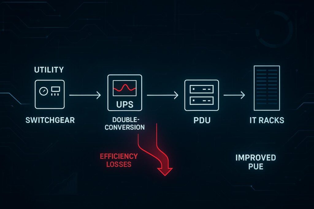
Lower cooling energy: every watt the UPS wastes becomes heat that cooling systems must remove.
What’s changed in the last decade is that modern UPS platforms increasingly combine high-frequency online double-conversion designs with dynamic online / high-efficiency operating modes, trying to keep strong power-quality protection while reducing conversion losses when conditions allow.
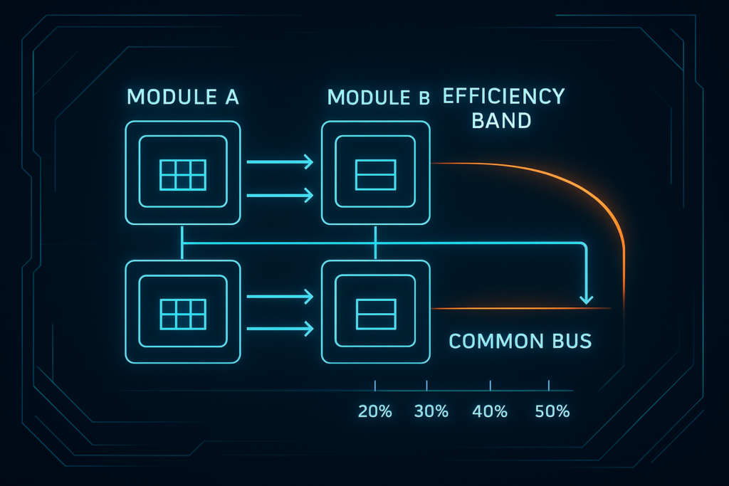
This article focuses on the part-load reality most operators live in: 20%–50% loading, driven by redundancy targets (N+1, 2N), phased buildouts, and uneven IT ramp. Efficiency ranges and examples use recent, commonly cited industry figures and conservative assumptions.
PUE and the UPS Loss Pathway (UPS efficiency lowers PUE)
Define PUE and UPS’s role in facility energy
PUE is the most widely used top-level metric for data center energy efficiency (data center PUE):
PUE = Total Facility Power ÷ IT Equipment Power
“Total facility” includes everything needed to support IT—power conversion, distribution losses, cooling, lighting, and auxiliaries—so the UPS sits squarely in the PUE numerator as infrastructure overhead. That’s why improving UPS efficiency can reduce data center PUE, even if nothing changes on the IT side.
How UPS losses raise the numerator and add heat
A UPS has an output (what your IT sees) and an input (what the facility must supply). Its efficiency is:
η = P_out ÷ P_in
If we treat the UPS output as the IT load it serves, the UPS electrical loss can be estimated as:
UPS loss (kW) ≈ IT load (kW) × (1/η − 1)
That loss increases total facility power immediately. But it also matters thermally: nearly all UPS losses end up as heat inside the building envelope.
As Rehlko notes in its explainer on UPS efficiency and PUE, improving UPS efficiency reduces the infrastructure overhead counted in PUE, and also reduces heat that must be removed by cooling systems, compounding the impact on facility energy use (Rehlko: “How UPS efficiency can contribute to data centre PUE”).
Cooling amplification and COP/EER linkage
Cooling systems have their own efficiency. A standard way to approximate how much additional electrical input is required to remove a given heat load is the coefficient of performance (COP):
Added cooling power (kW) ≈ Added heat load (kW) ÷ COP
So if UPS losses add 20 kW of heat and your marginal COP is 4, the cooling plant might need ~5 kW more electrical input to remove that heat. That means a UPS loss is rarely “just” an electrical penalty—it’s often an electrical penalty plus a cooling penalty.
A compact way to express the UPS contribution to PUE is:
ΔPUE_from_UPS_losses ≈ (UPS loss ÷ IT load) × (1 + 1/COP)
The exact number depends on where the heat is rejected (UPS room vs white space), your cooling architecture, and seasonal conditions. But the direction is consistent: higher UPS efficiency reduces facility overhead twice.
Modern UPS Efficiency Ranges
Legacy double-conversion baselines and limits
Traditional double-conversion UPS topologies are valued because they deliver consistent output and isolate the IT bus from many upstream disturbances. The tradeoff has historically been conversion loss.
A practical engineering summary is that double-conversion efficiency rises with load, and legacy/static designs can be notably less efficient at light loads. Consulting-Specifying Engineer summarizes typical double-conversion performance as roughly ~90% at ~30% load and ~94% at full load, noting that specific implementations (including isolation transformers) can move the curve (Consulting-Specifying Engineer: “Evaluating UPS system efficiency”).
High-frequency online double-conversion today
Modern online UPS designs increasingly use high-frequency power conversion (often with transformerless architectures) to reduce losses and improve part-load behavior. The key point for a buyer isn’t the headline peak efficiency—it’s the efficiency at your operating point, which in many redundant facilities lands in the 20%–50% band.
In practice, you’ll see modern online double-conversion UPS platforms publish higher “true online” efficiency than older generations, but the curve shape still matters: no-load and light-load overheads can dominate when systems are oversized.
Dynamic online/high-efficiency modes explained
Many UPS platforms now include energy-saving modes (often branded as “eco,” “dynamic,” or “high-efficiency” modes). The basic idea is to reduce how much power continuously flows through the full conversion chain when input power quality is acceptable.
That can raise efficiency meaningfully, but it introduces a procurement-relevant question: what are the performance tradeoffs (transfer behavior, disturbance tolerance, and power-quality bounds) under this mode? As one engineering overview notes, with rectifier/inverter losses reduced or bypassed, eco modes can push UPS efficiency into the high 90s, but the load may be more exposed to utility events depending on implementation.
Partial-Load Realities and Optimization (partial-load UPS efficiency)
Redundancy impacts and 20%–50% loading behavior
If you operate with redundancy, your UPS rarely runs at a tidy “best efficiency point” all the time.
In N+1, you intentionally install more capacity than strictly needed, so the system can lose a module/block and still carry the load.
In 2N, each side is typically constrained to operate below ~50% so that either path can carry the full load during a failure or maintenance event.
The result: many sites spend long periods at 20%–50% loading, especially during phased buildouts or uneven IT ramp. Coolnetpower’s breakdown of redundancy tiers is a useful way to frame this as a design requirement rather than a label (Coolnetpower: “N+1 vs 2N redundancy tradeoffs”).
For a more complete sizing workflow—including how to translate measured IT kW into UPS capacity, apply redundancy, and then validate efficiency at the real load point—see Coolnetpower’s PUE calculation workflow.
Intelligent paralleling and right-sizing modules
If light-load operation is your reality, the efficiency lever is often how you implement capacity, not only which topology you choose.
Two practical tactics show up repeatedly in efficient facilities:
Right-size to the ramp plan: size the UPS to the IT load you will actually energize in the next phase, with an explicit growth assumption and a redundancy target.
Use modular capacity with intelligent paralleling: keep fewer modules active at low load so the active modules operate in a higher-efficiency band, while still maintaining redundancy.
A good procurement habit is to demand efficiency curves (or verified performance data) at the same load points you will operate at—commonly 25%, 50%, 75%, 100%—and to validate whether those curves assume any special mode.
Coolnetpower’s right-sizing workflow is useful here because it treats capacity selection as a repeatable process: measure, convert, apply margin and topology, then validate runtime and efficiency at the real operating point (Coolnetpower: “how to right-size a UPS for efficiency”).
In this section, that’s the practical meaning of partial-load UPS efficiency: you’re managing efficiency by managing how much capacity is online at any time—not just buying a higher-number datasheet.
Safe use of high-efficiency modes under power quality bounds
High-efficiency modes can be a legitimate lever—but only if the facility’s risk posture and power-quality environment support it.
In practice, “safe” enablement tends to require:
Defined input bounds (voltage/frequency windows, harmonic limits) that trigger a return to full online protection when exceeded
Clear transfer behavior (how quickly the UPS transitions, and what events can cause a transfer)
Coordination with generators and switchgear (to avoid nuisance transfers or unintended ride-through gaps)
Where Coolnetpower’s experience fits (informational): in many U.S. builds and expansions, the hardest operating window is not peak load—it’s the 20%–50% ramp period where redundancy is already installed but IT load hasn’t fully arrived. Engineering attention to high-frequency online double-conversion design and module-level paralleling control can help keep output power quality stable while reducing the “part-load penalty” that otherwise shows up in PUE and cooling.
Quantifying PUE and Cost Impact
Back-of-the-envelope method and key formulas
To estimate the impact of improving UPS efficiency at a given IT load:
UPS loss (kW)
UPS loss ≈ IT × (1/η − 1)
Added cooling power (kW) (approximate)
Added cooling ≈ UPS loss ÷ COP
Total facility delta (kW) from UPS efficiency change
ΔFacility ≈ (UPS loss_old − UPS loss_new) × (1 + 1/COP)
Annual energy (kWh)
Annual kWh ≈ ΔFacility (kW) × 8,760
Annual $
Annual $ ≈ Annual kWh × electricity price ($/kWh)
Key Takeaway: For most facilities, the “value” of UPS efficiency is bigger than the nameplate percent change because you avoid both electrical losses and the cooling energy needed to remove the resulting heat.
Example calculation: 1 MW facility scenario
Assumptions (hypothetical, for sizing intuition):
IT load served by UPS: 1.0 MW (1,000 kW)
UPS efficiency improves from 94% to 97% at the actual operating point
Marginal cooling COP: 4.0
Electricity price: $0.10/kWh
Constant load for simplicity (real sites vary)
Step 1: UPS losses
At 94%: loss ≈ 1,000 × (1/0.94 − 1) ≈ 63.8 kW
At 97%: loss ≈ 1,000 × (1/0.97 − 1) ≈ 30.9 kW
Loss reduction ≈ 32.9 kW
Step 2: include cooling amplification
ΔFacility ≈ 32.9 × (1 + 1/4) ≈ 41.1 kW
Step 3: annualize
Annual kWh ≈ 41.1 × 8,760 ≈ 360,000 kWh
Annual $ ≈ 360,000 × $0.10 ≈ $36,000/year
What this means for PUE
ΔPUE_from_UPS ≈ (32.9/1,000) × (1 + 1/4) ≈ 0.041
That’s not a promise—it’s a sensitivity estimate. Your actual COP, duty cycle, and operating mode will move it.
Example calculation: 5 MW facility scenario
Using the same assumptions but scaling IT load to 5 MW:
Loss reduction scales roughly with IT load: 32.9 kW × 5 ≈ 164.5 kW
ΔFacility ≈ 164.5 × 1.25 ≈ 205.6 kW
Annual kWh ≈ 205.6 × 8,760 ≈ 1,801,000 kWh
Annual $ ≈ 1,801,000 × $0.10 ≈ $180,000/year
In larger sites, the operational value can also show up as avoided strain on electrical and cooling capacity during expansion phases.
Selection and Operational Guidance
Protection, transfer behavior, and power quality criteria
For an awareness-stage buyer, the most useful question isn’t “what is the highest efficiency?” It’s:
What efficiency can you achieve at 20%–50% load without violating your power-quality and transfer requirements?
Practical evaluation criteria to document early:
Topology and performance class: confirm what “online” means in the vendor’s terminology and what disturbances are corrected vs passed through.
Mode definitions: define the conditions for entering/exiting high-efficiency modes.
Transfer behavior: understand what events trigger a transfer and whether there is any non-zero transfer time in your chosen mode.
Generator interaction: verify stability during generator starts, load steps, and frequency excursions.
Monitoring, metering, and verifying savings in live ops
If you want efficiency improvements to show up in a PUE report, you need measurement discipline:
Meter at the right points: input to UPS, output from UPS, and cooling energy for the UPS room/zone where applicable.
Use time alignment: compare like-to-like operating windows (similar IT load and similar seasons).
Track operating mode: log when the UPS is in online vs high-efficiency/eco modes so you don’t attribute savings to the wrong cause.
This is also how you avoid “paper efficiency” that disappears in real operation because the UPS spends most of its time outside the assumed mode.
Deployment roadmap and risk mitigation steps
A conservative rollout approach that fits compliance-sensitive environments:
Baseline: collect two to four weeks of UPS input/output and thermal data.
Model: run the back-of-the-envelope estimate with your real loading distribution (how many hours at 20%, 30%, 40%, 50%).
Pilot: enable any high-efficiency mode in a limited scope with defined trip thresholds and rollback criteria.
Validate: confirm no increase in transfer events, alarms, or power-quality excursions.
Standardize: document settings, thresholds, and commissioning tests so the result survives staff changes.
If you want a procurement-friendly starting point, you can request a commissioning and metering checklist that ties UPS mode settings to measurable acceptance criteria.
Conclusion
UPS efficiency lowers PUE in two ways: it reduces direct electrical losses counted in total facility power, and it reduces cooling energy by cutting the heat those losses create.
In modern data centers, the biggest gains often come from aligning the UPS’s real operating point—commonly 20%–50% load—with the efficiency curve you will actually achieve under your redundancy and power-quality requirements. Dynamic online controls and modular paralleling strategies can help, but they need to be validated against transfer behavior and site power conditions.
For U.S. buyers, the practical takeaway is straightforward:
Ask for efficiency at your real loading band (not just peak numbers).
Treat high-efficiency modes as an engineering decision with defined risk bounds.
Verify savings with metering that separates UPS losses from cooling impacts.